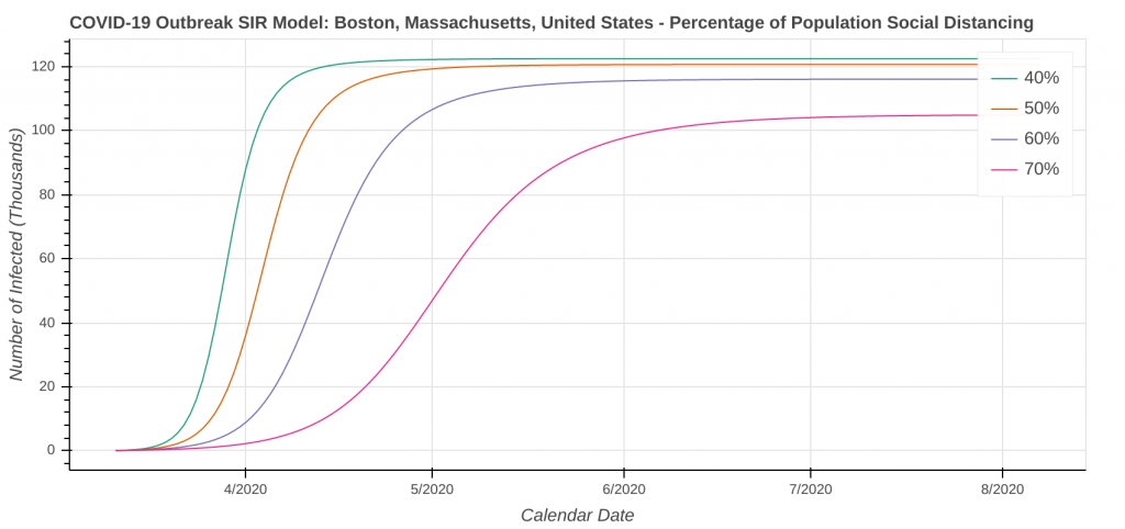
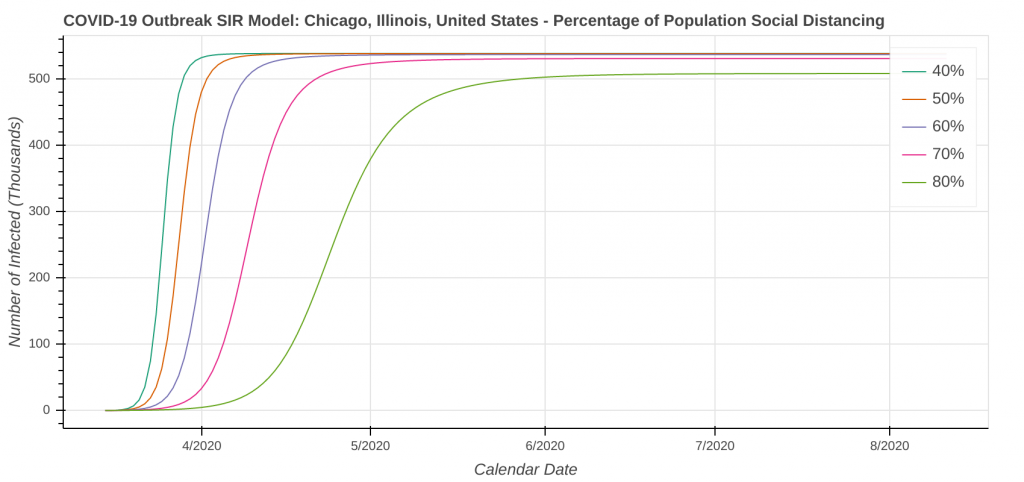
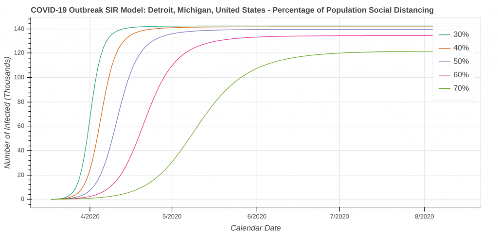
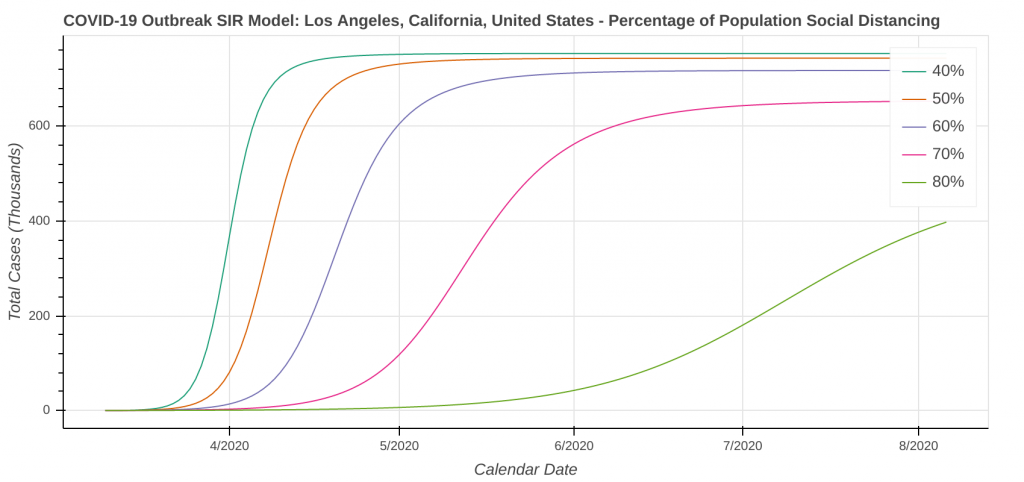
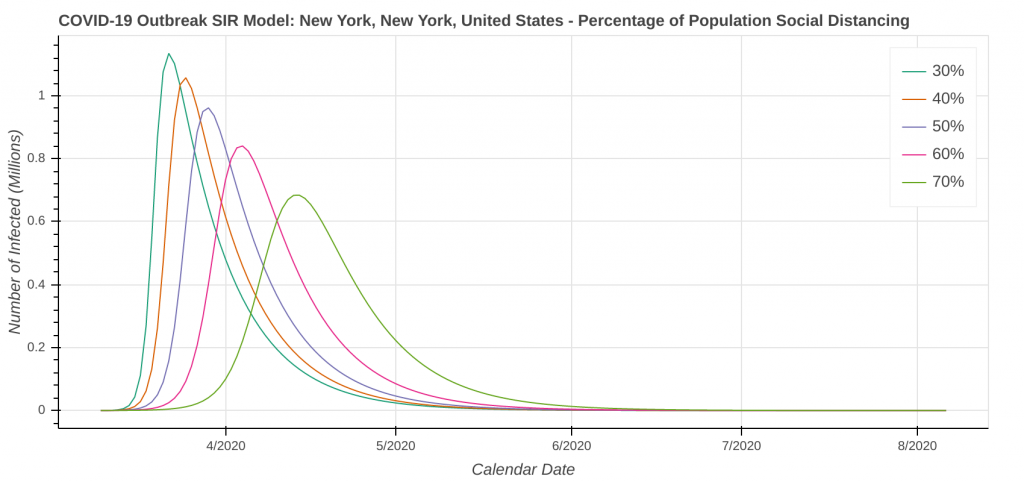
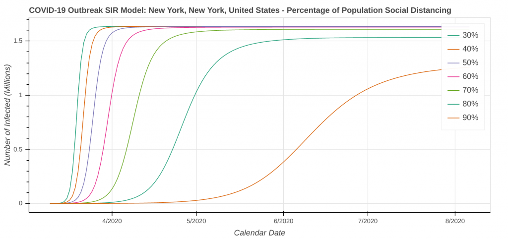
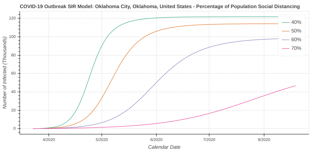
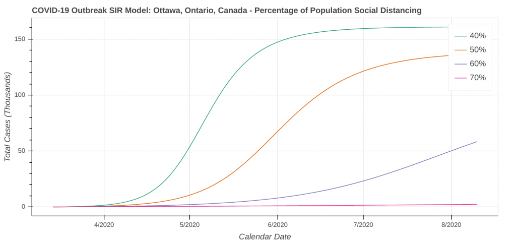
Here is a full look at the outputs from our revised SIR model. I have included plots from hot spots in both the US and Canada as well as cities where I have friends, family, and loved ones. I can run these simulations for just about any city in the world, so if you have any cities you want to see, leave me a message in the comments or contact me directly.
Overview of SIR Model Output
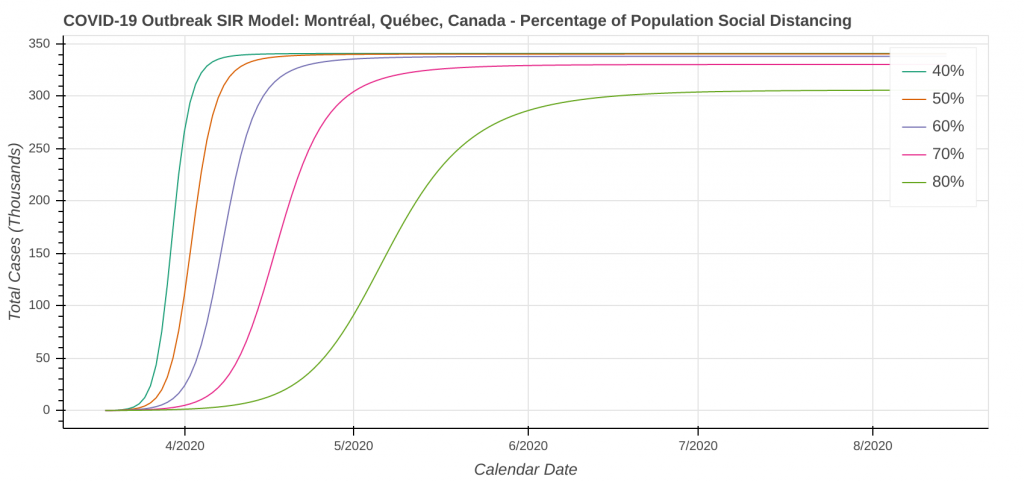
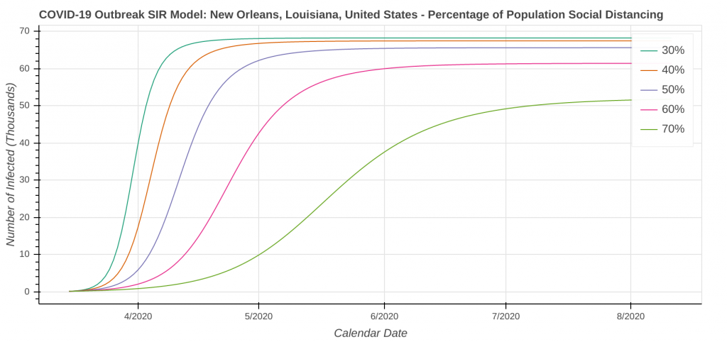
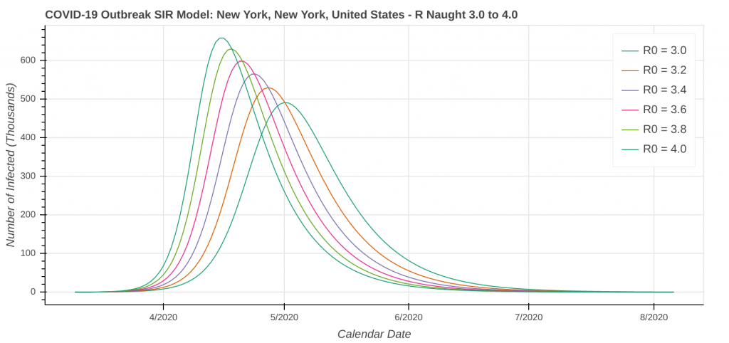
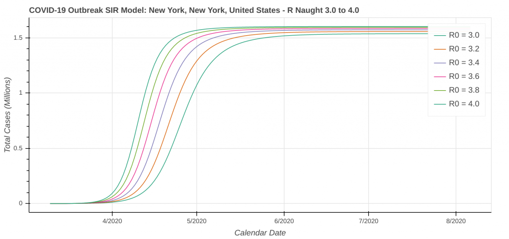
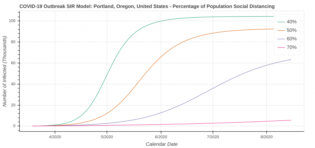
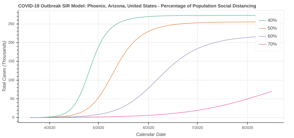
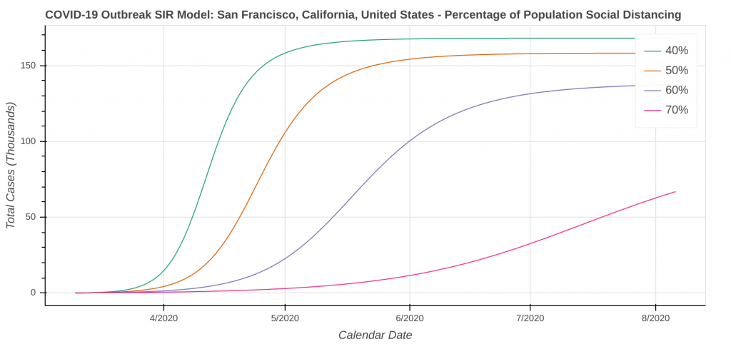
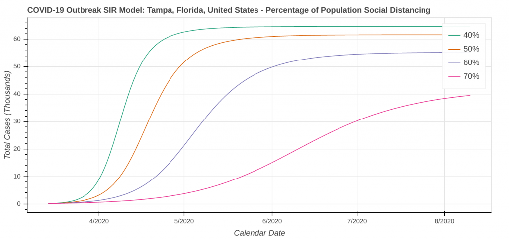
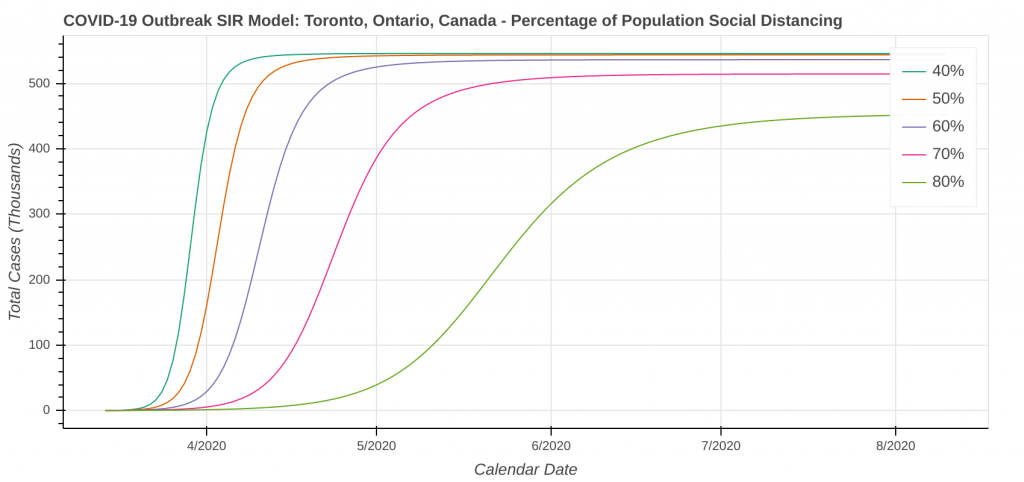
Each city has four plots. The top row is the “working” model output, with the model curve best fit to the actual data. The bottom row is an experimental model output showing the effect of social distancing. In the “working” model runs on the top row, there are 5 lines on each plot. The middle line is the R Naught value that was reverse-engineered by fitting the model output to the actual data, and there are two lines on each side of the best-fit line showing different R Naught values in steps of 0.2.
Note: The y-axis on some of the experimental social distancing plots showing the total case count (bottom right plot for each city) is mislabeled. It should read “Total Cases”, not “Number of Infected”.
Finally, don’t forget that the plots below assume the R Naught values and the amount of social distancing remains constant throughout the entire time series. In reality, additional social distancing restrictions will dampen the curve and shift it to the right, while removing social distancing restrictions will cause the curve to accelerate and shift to the left.
Confidence in SIR Model Predictions
My confidence level in the “working”/top row model outputs is as follows:
- Predicting the apex of the outbreak: medium-high to high. The curves should at least be “in the ballpark.”
- Predicting the total number of cases: low to very low. With how fast things are changing right now and how fast new data is coming in, we just don’t know at this point. My gut feeling is that the case count projections in these model runs are likely high overall, but from a public health perspective, I would much rather have the model overestimate case counts than underestimate them.
Plots are in alphabetical order by city, with a table of additional cities at the bottom. Click on any plot to view it full size.
Boston, Massachusetts
Chicago, Illinois
Detroit, Michigan
Los Angeles, California
Montréal, Québec
New Orleans, Louisiana
New York, New York
Oklahoma City, Oklahoma
Ottawa, Ontario
Portland, Oregon
Phoenix, Arizona
San Francisco, California
Tampa, Florida
Toronto, Ontario
SIR Model Outputs for Additional Cities
Please note that this table contains outputs of just this single model run and does not necessarily reflect what my actual predictions are. I will be putting this table on my COVID-19 Pandemic Tracker later this week and regularly updating it there.
Data points I’m skeptical of in this output (with some comments):
- Chicago, IL: Case count is likely overestimated. I’m not sure why, but the most likely reason is good social distancing.
- Los Angeles, CA: Case count is likely overestimated due to California being better at social distancing than what was input into the model
- Seattle, WA: Peak date is incorrect due to the State of Washington’s 100th case occurring before John’s Hopkins began breaking down data by state.
- Washington, DC: Not enough data to accurately fit the curve
- Winnipeg, MB: Not enough data to accurately fit the curve
| City | State or Province | Apex Date | Total Cases @ Apex | Infected @ Apex |
|---|---|---|---|---|
| Atlanta | Georgia | Late April to Early May | 10,000 to 100,000 | 10,000 to 100,000 |
| Boston | Massachusetts | Late April to Early May | 50,000 to 200,000 | 10,000 to 50,000 |
| Calgary | Alberta | Early June | 10,000 to 100,000 | 10,000 to 50,000 |
| Chicago | Illinois | Mid-to-Late April | 100,000 to 500,000 | 100,000 to 200,000 |
| Dallas | Texas | Early May | 100,000 to 500,000 | 50,000 to 100,000 |
| Denver | Colorado | Early-to-Mid May | 10,000 to 100,000 | 10,000 to 50,000 |
| Detroit | Michigan | Mid-to-Late April | 50,000 to 100,000 | 10,000 to 100,000 |
| Edmonton | Alberta | Late May to Early June | 10,000 to 100,000 | 10,000 to 50,000 |
| Houston | Texas | Early May | 100,000 to 500,000 | 50,000 to 150,000 |
| Los Angeles | California | Early May | 100,000 to 1,000,000 | 100,000 to 500,000 |
| Miami | Florida | Late April | 10,000 to 100,000 | 10,000 to 50,000 |
| Montréal | Québec | Late April to Early May | 100,000 to 500,000 | 10,000 to 100,000 |
| New Orleans | Louisiana | Mid-to-Late April | 10,000 to 100,000 | 10,000 to 50,000 |
| New York | New York | Mid-April | 100,000 to 1,000,000 | 100,000 to 700,000 |
| Oklahoma City | Oklahoma | Early-to-Mid May | 10,000 to 100,000 | 10,000 to 50,000 |
| Ottawa | Ontario | Mid May | 50,000 to 200,000 | 10,000 to 50,000 |
| Philadelphia | Pennsylvania | Late April to Early May | 50,000 to 500,000 | 50,000 to 100,000 |
| Phoenix | Arizona | Mid May | 10,000 to 200,000 | 10,000 to 100,000 |
| Portland | Oregon | Late May to Early June | 10,000 to 100,000 | 5,000 to 50,000 |
| Seattle | Washington | Late April to Early May | 10,000 to 100,000 | 10,000 to 50,000 |
| San Francisco | California | Late April to Early May | 50,000 to 200,000 | 10,000 to 50,000 |
| Tampa | Florida | Mid-to-Late April | 10,000 to 100,000 | 10,000 to 50,000 |
| Toronto | Ontario | Mid-to-Late May | 100,000 to 500,000 | 50,000 to 200,000 |
| Vancouver | British Columbia | Early to Mid June | 10,000 to 100,000 | 5,000 to 50,000 |
| Washington | District of Columbia | Late May to Early June | 10,000 to 100,000 | 10,000 to 50,000 |
| Winnipeg | Manitoba | Late June to Early July | 10,000 to 100,000 | 1,000 to 20,000 |


